State Reduction
The three main methods of state reduction include:
Row matching
Row matching, which is the easiest of the three, works well for state transition tables which have an obvious next state and output equivalences for each of the present states. This method will generally not give the most simplified state machine available, but its ease of use and consistently fair results is a good reason to pursue the method.
Implication charts
The implication chart uses a graphical grid to help find any implications or equivalences and is a great systematic approach to reducing state machines.
Successive partitioning
Successive partitioning is almost a cross between row matching and implication chart where both a graphical table and equivalent matching is used.
Each of these methods will, in most cases, reduce a state machine into a smaller number of states. Keep in mind that one method may result in a simpler state machine than another. Experience will help in understanding and determining the best method to use in any particular situation.
Row Matching
The row matching method, as previously described, is the quite possibly the simplest of the three methods. It uses the state equivalence theorem: Si = Sj if and only if for every single input X, the outputs are the same and the next states are equivalent (Grover, 2007). All input sequences must be considered, but any information about the internal state of the system can be ignored. When using the theorem, both the output and next state must be considered. However, only single inputs rather than input sequences are considered. The typical recipe for reducing in the row reduction method is
An example can be seen by observing Table 1 below:
The row matching method, as previously described, is the quite possibly the simplest of the three methods. It uses the state equivalence theorem: Si = Sj if and only if for every single input X, the outputs are the same and the next states are equivalent (Grover, 2007). All input sequences must be considered, but any information about the internal state of the system can be ignored. When using the theorem, both the output and next state must be considered. However, only single inputs rather than input sequences are considered. The typical recipe for reducing in the row reduction method is
- Start with the state transition table
- Identify states with same output behavior .
- If such states transition to the same next state, they are equivalent
- Combine into a single new renamed state
- Repeat until no new states are combined
An example can be seen by observing Table 1 below:
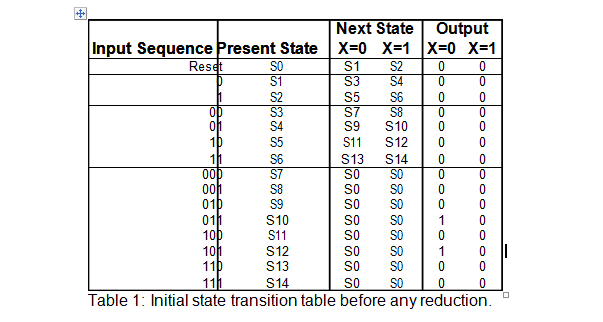
First, notice that S10 and S12 have the same next states as well as the same outputs.
These two states can be combined and renamed into S10' (the tick mark ' signifies that this state has been merged with another and is considered a new, reduced state).
Because S12 no longer exists, all instances of S12 will be replaced with S10'. This will result in Table 2 below:
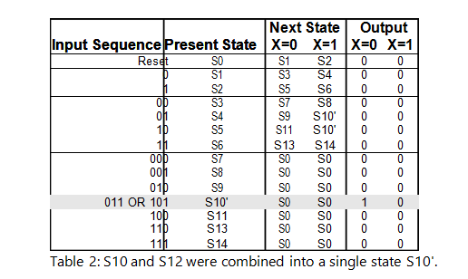
This process is continued until no new states can be combined. The resulting table can be seen below in Table 3:
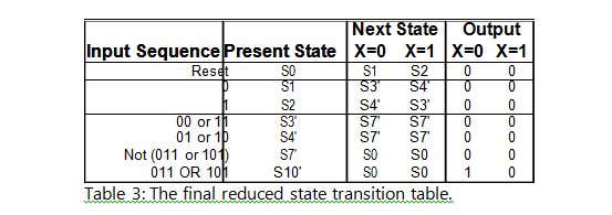
In this particular example, the number of states was reduced from fifteen (15) to seven (7) states. This literally amounts to a reduction of eight (8) states and the elimination of one flip-flop for the final design.
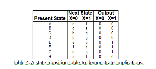
Implication Chart Method
The implication chart method uses a graphical grid of sorts to systematically find equivalences among the states. The implication chart assists in keeping track of any implications such as, for example, c-d and e-f are implied pairs for a-b in Table 4 below:
Implication Chart Method
The implication chart method uses a graphical grid of sorts to systematically find equivalences among the states. The implication chart assists in keeping track of any implications such as, for example, c-d and e-f are implied pairs for a-b in Table 4 below:
Focusing attention towards a different example, the implication chart method will be demonstrated in more detail. The steps that need to be taken in this method can be summed up into a recipe.
1.Construct implication chart, one square for each combination of states taken two at a time .
2.Square labeled Si, Sj, if outputs differ then the square gets an 'X'. Otherwise, write down implied state pairs for all input combinations .
3.Advance through chart top-to-bottom and left-to-right. If square Si, Sj contains next state pair Sm, Sn and that pair labels a square already labeled 'X' then Si, Sj is labeled 'X' .
4.Continue executing Step 3 until no new squares are marked with 'X' .
5.For each remaining unmarked square Si, Sj, then Si and Sj are equivalent .
Consider the following transition table:
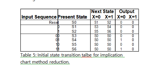
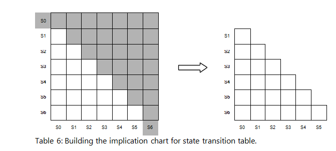
The first step is to construct an implication chart which can be seen in Table 6 below:
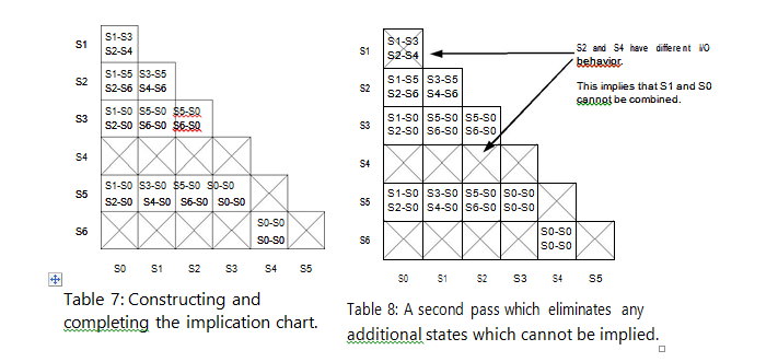
Construction of the implication chart also includes filling in the values of the state transition table as seen in Table 7 below. Notice the 'X's where the outputs of the compared states are different, this is done in step 2. In step 3, which is demonstrated in Table 8, will further eliminate any states which cannot be implied.
Step 4 is to repeat the processes of step 3 until no more comparisons can be made. The final result is what is left over after this step is completed. The final implication chart and transition table can be seen below in Tables 9 and 10.
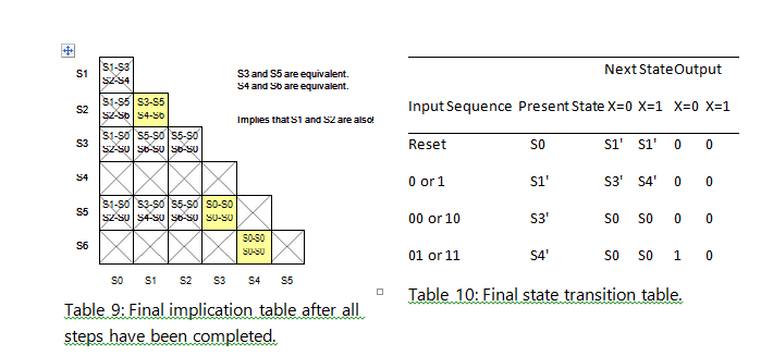
In this particular example, the implication chart method simplified the state transition table from seven (7) states down to five (5) states.
Partitioning Method
As mentioned before, the partitioning method is a sort of hybrid between row matching and implication chart in that it uses a visual detection for equivalences as well as a chart to organize the process. Partitioning provides a straightforward procedure for determining equivalency for any amount of complexity. Successive partitioning steps produce smaller partitions. If the next step does not yield any smaller partitions no further steps will yield any smaller partitions and, hence, the partitioning process is then complete. All states that are in the same partition after k steps are k equivalent. All states that are in the same partition when no further partitioning can be accomplished are equivalent. States that are not in the same final partition are not equivalent.
The following state transition table example will be used to demonstrate the partitioning method:
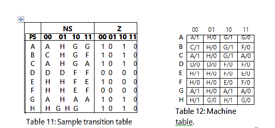
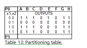
In order to start this reduction method, it is beneficial to convert the transition table into a machine table which will make it easier to transfer to the partition table. This is an optional step, but it will save a little time in the long run. Refer to Table 12. The rows of this machine table are the state names from the transition table. The columns are the next state conditions. The values within the cells are in the form next state/output. The next step is to transfer the information into the partitioning table as seen in Table 13 below:
As illustrated in Table 15, the next step is to find any of the outputs which are the same, and then partition them off (or group them into a partition) and record these in the P1 row (which basically stands for partition pass 1). The next step is to replace the outputs with the next state names and then determine if any of the states need to be partitioned out. In order to tell this, if states within the column being observed are not within the partition, then it should be partitioned off (as seen Table 14). After repeating this step for all columns and partitions, the final partition table can be seen in Table 17. The composite table with all of these steps combined can be seen in Table 16.
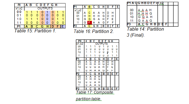
From the final step in the partition table, the states left grouped in the partitions are all equivalent. In this case, the equivalences are as follows:
A' = A = C = G = H F
B' = B
C' = D
D' = E
E' = F
The final step is to put the results of the successive partitioning method back into either the state transition table or the state machine table as seen in Tables 18 and 19 below:
A' = A = C = G = H F
B' = B
C' = D
D' = E
E' = F
The final step is to put the results of the successive partitioning method back into either the state transition table or the state machine table as seen in Tables 18 and 19 below:
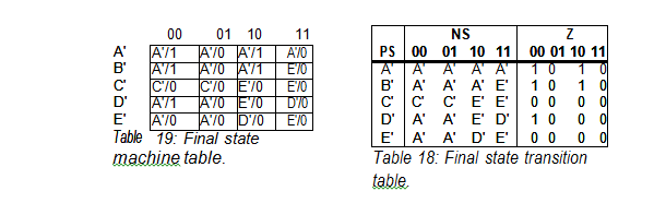
In this particular example, the number of states was reduced from seven (7) states to five (5) states.
